WPS offers a useful feature called crosshairs, which highlights the rows and columns of selected cells. This is particularly helpful when working with large datasets, as it makes it easier to track your data. Unfortunately, Excel does not include this feature natively. After some research, I discovered that a similar effect can be achieved using VBA, so I decided to give it a try.
The approach involves using VBA to identify the rows and columns within the selected range, then applying conditional formatting to highlight them. Whenever the selection changes, the code clears any existing conditional formatting, reapplies the highlights to the new selection, and updates the fill color accordingly.
The main limitation of this method is that it relies on conditional formatting for highlighting. As a result, if you enable this feature, you won’t be able to use other conditional formatting rules in the table because the code clears all conditional formatting each time the selection changes.
Here is the VBA code used:
Private Sub Worksheet_SelectionChange(ByVal Target As Range)
    Cells.FormatConditions.Delete ' Clear existing conditional formatting
    For Each Row In Target.Rows ' Iterate over selected rows
        With Row.EntireRow.FormatConditions ' Apply conditional formatting to the row
            .Delete
            .Add xlExpression, , "TRUE"
            .Item(1).Interior.Color = RGB(217, 217, 217)
        End With
    Next
    For Each Col In Target.Columns ' Iterate over selected columns
        With Col.EntireColumn.FormatConditions ' Apply conditional formatting to the column
            .Delete
            .Add xlExpression, , "TRUE"
            .Item(1).Interior.Color = RGB(217, 217, 217)
        End With
    Next
End Sub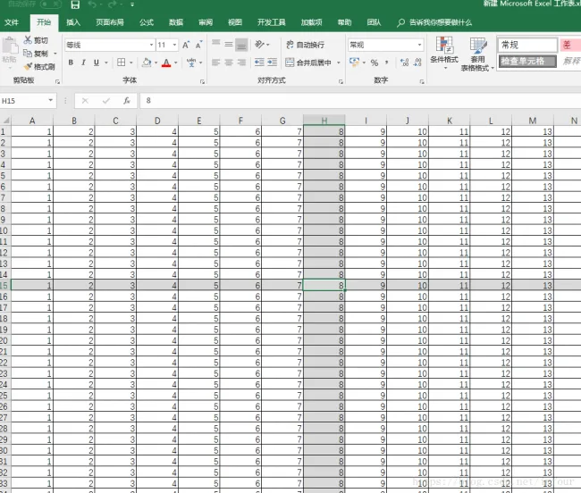


Must log in before commenting!
Sign Up