A new entrance and exit road will be constructed in a mountainous scenic area. The road features a single slab cross-section with a 9-meter-wide roadbed. The pavement structure consists of 4cm fine-grained asphalt concrete (AC-13) over 6cm medium-grained asphalt concrete (AC-20). A seal coat of emulsified asphalt will be applied as a lower seal coat. The grassroots layer will be made of 20cm of 5% cement-stabilized crushed stone, resting on a 40cm mountain soil base. Shoulder drainage ditches will be installed along both sides of the road. To enhance the landscape, camphor trees will be planted on each side of the road shoulders, positioned 4m from the centerline and spaced every 7m, creating a tree-lined avenue.
1) Calculating Roadbed and Pavement Quantities Using the Average Cross-Section Method
A. Preparing the Data Source
Before calculating quantities with the average cross-section method, create a terrain surface. Following standard design procedures, establish the road plan alignment, vertical profile, and cross-sectional assemblies sequentially. Generate a road model on the terrain surface, then right-click the model to access road properties (see Figure 1). Extract specific surfaces such as the road top surface (Top) and a reference surface (Datum) from this model. The Datum surface represents the bottom of the pavement structure layer, the top of the roadbed, and slopes, and is used to calculate earthwork volumes excluding the pavement structure.
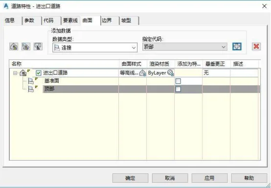
Figure 1: Creating specified surfaces Top and Datum from the road model
B. Setting Sampling Lines
Sampling lines enable cross-sectional sampling on data sources such as the original terrain surface, road model entities, and specified road surfaces. Each data source generates a cross-sectional line, which helps calculate the excavation area at each station.
Use the command to create sampling lines in the sampling line toolbar, specifying the mileage range, sampling width, and line accuracy as shown in Figure 2. Straight segments can be divided into 20-meter intervals, while curves, gentle bends, or areas with significant terrain changes require denser sampling. Increasing sampling density in these sections improves earthwork quantity accuracy.
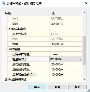
Figure 2: Dialogue box for setting sampling line parameters
C. Customizing Earthwork and Rock Standards
Open the Toolspace Settings tab and access the Quantity Standards dialog box (see Figure 3). Here, configure calculation methods for soil and rock loosening coefficients, fill and excavation volumes, and pavement structure materials. Excavation volume refers to the portion below the natural ground surface but above the designed curved surface; anything else is considered fill. Pavement structure layer codes correspond to the road material shape codes in the cross-sectional assembly, including surface, base, and subbase layers.
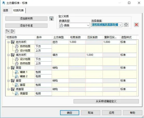
Figure 3: Earthwork standard setting dialog box
D. Calculating Roadbed and Pavement Engineering Quantities
Navigate to the Analysis tab and run the Calculate Material command. Select the route and corresponding sampling line group to be analyzed, then open the Edit Material List dialog box. Import or modify calculation rules as needed.
In the material calculation dialog, set the earthwork standard and choose “average end area” as the volume calculation method. Specify surfaces and modeling objects as shown in Figure 4: the natural surface corresponds to the original terrain, and the design surface is the Datum extracted from the road model. Pavement 1 represents the upper layer, Pavement 2 the lower layer, with base and subbase layers defined accordingly. After specifying these, return to the Sampling Line Group Properties dialog, expand the Material List, and review all objects slated for calculation.
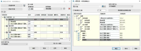
Figure 4: Dialog box for specifying calculation materials
Use the Volume Report command under the Analysis tab to specify the route, sampling line group, and material list. Select the Material style sheet to view the calculated earthwork and pavement structure quantities, as shown in Figures 5 and 6.
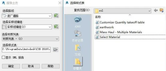
Figure 5: Dialog box for outputting material calculation results
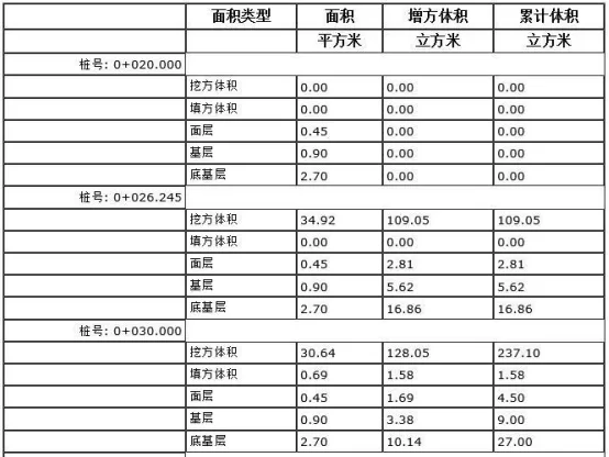
Figure 6: Material calculation results report
E. Outputting the Results
Engineering quantity results can be output as tables formatted for bill of quantities. Use the command to create a total volume table, selecting the route and sampling line group to be reported. This generates an earthwork calculation table, as illustrated in Figure 7.
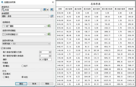
Figure 7: Output of earthwork calculation results table
Click the “Create Material Volume Table” command to generate separate tables for earthwork filling, excavation, and each pavement structure layer. Figure 8 shows the base volume calculation table detailing area and volume results for the pavement base structure, complying with bill of quantities unit requirements.
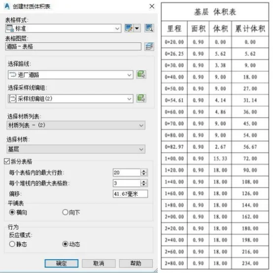
Figure 8: Calculation results of pavement base engineering quantity
2) Calculating Roadbed and Pavement Quantities Using the Volume Surface Method
The accuracy of the average cross-section method depends on sampling line density. According to integration principles, infinitely increasing sampling line density approximates the volume surface method—creating benchmark surfaces (terrain surface) and reference surfaces (road design surface), then subtracting the soil volume between them.
Select the terrain surface and extract entities from it. Set the extraction target to the road reference surface (Datum) to create a volume entity representing earthwork filling and excavation between the pavement bottom and terrain. Convert this volume entity into a volume element by right-clicking it. The precise volume can be viewed in the object properties, as shown in Figures 9 and 10. Similarly, different pavement structure layers can be analyzed by selecting their respective surfaces.
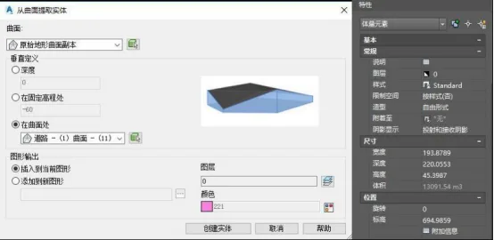
Figure 9: Mass element calculation dialog box
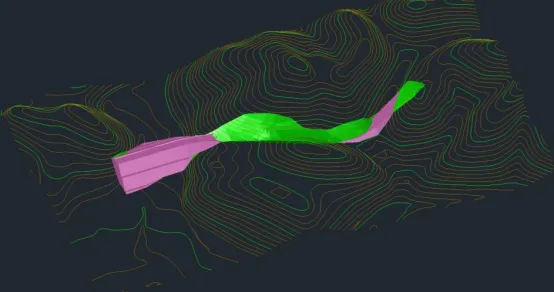
Figure 10: Volume element calculation effect diagram
3) Calculating Clearing Quantities
To calculate filling and clearing quantities, first identify the fill section boundaries. Select the original terrain surface and run the “Minimum Distance between Surfaces” command, selecting the terrain surface and road reference surface consecutively. This yields the boundary line between the original terrain and the road reference surface, which distinguishes fill from excavation areas.
Create a copy of the original terrain surface and add the boundary line on the fill side as the terrain surface boundary. This new surface defines the required fill section clearing range, as shown in Figure 11.
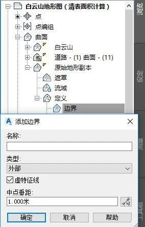
Figure 11: Define surface external boundary dialog box
Select the fill and clearing surface, open its properties dialog box, and expand the statistics section to view both 2D and 3D surface areas, as shown in Figure 12.
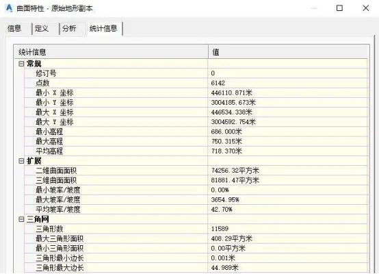
Figure 12: Surface information query dialog box
4) Calculating Side Ditch Quantities
The cross-section of the side ditch is fixed, and its quantity is calculated based on mileage length for the bill of quantities. After generating the road model, run the command to extract road feature lines, selecting the required lines. This creates a 3D polyline representing the side ditch (see Figure 13). Querying its properties reveals both the 2D projected length and the 3D spatial length of the ditch feature line.
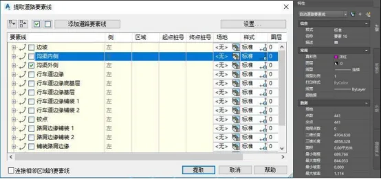
Figure 13: Dialogue box for extracting road feature lines
5) Calculating Greening Quantities
Plant layouts are created by placing points styled to represent plant shapes. In the Toolspace Settings dialog, expand the Point Styles tab and create a new style named “Cinnamomum camphora.” Open the point style settings and set the representation to a 3D camphor tree model, as shown in Figure 14.
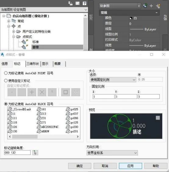
Figure 14: Point style creation and setting dialog box
For easier management, group similar structures in a point group. Use the ‘Create Point Group’ command, name it “Camphor Point Group,” and assign the Camphor point style, as seen in Figure 15.
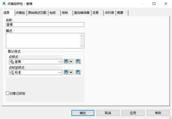
Figure 15: Dialogue box for creating and setting point grouping
Use the ‘Create Point’ command to generate points along the route by distance. Specify the route for the project and set start and end station numbers. Set an offset distance of 4m from the centerline and spacing of 7m between points. After creation, right-click to select similar points, select all camphor points, and use the command to assign elevations from the road top surface, completing the tree layout along the road. A partial view is shown in Figure 16.
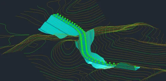
Figure 16: Layout effect of camphor trees along the route
Open the Toolspace palette and browse the point groups to clearly see the total number of camphor trees within the Camphor Point Group, as shown in Figure 17.
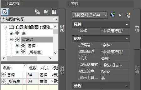
Figure 17: Command bar for querying engineering quantities through point grouping


Must log in before commenting!
Sign Up